
Project
Finding suspicious devices in firewall logs
Six Python detection rules that turn a day of normal traffic into a baseline, then explain which devices deserve a closer look.
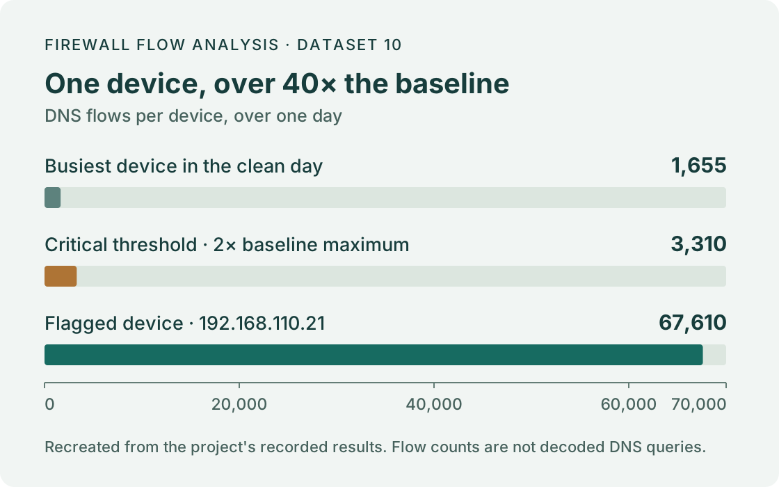
One device in the test data made 67,610 DNS flows in a day. The busiest device in the clean baseline made 1,655. That is an easy difference to spot once the right quantities are compared. Getting to that comparison was the work behind this project.
I implemented the analysis in Python and pandas in 2025, as a project submitted with Gonçalo Cunha for Security in Communications Networks at the University of Aveiro. My work covered profiling the firewall records, establishing a baseline, and writing all six detection rules. The result is a Jupyter notebook that identifies unusual activity and prints the measurements behind each finding.
The chart above was recreated for this article from the recorded dataset-10 results. It compares flow counts, including the rule’s critical threshold of twice the baseline maximum.
Start with an ordinary day
The assignment supplied three captures: a clean day of internal traffic, another day to investigate, and external clients accessing the company’s public servers. Each flow records a timestamp, source and destination addresses, protocol, destination port, and uploaded and downloaded bytes. There are no packet payloads or DNS query names.
The notebook defaults to dataset 10. Its baseline contains 964,901 flows from 197 internal source addresses. Looking at private destinations and their services identifies six internal servers: four serving HTTPS and two serving DNS.
HTTPS accounts for 88.1% of the baseline flows. A typical device uploads roughly one byte for every nine it downloads, and the middle 90% of devices make between 6.49 and 8.44 HTTPS flows per DNS flow. Those observations provide useful reference points. A device uploading ten times what it downloads deserves attention in this network, even though heavy uploads could be ordinary in a different setting.
Six ways to ask what changed
The first implementation used broader checks for traffic changes, ports, countries, and timing. The notebook develops six more specific rules:
| Rule | What it compares |
|---|---|
| Internal communication | Flow volume between internal pairs, and connections to destinations absent from the baseline server set |
| HTTPS upload ratio | Uploaded bytes divided by downloaded bytes for each source |
| HTTPS/DNS balance | The number of HTTPS flows relative to DNS flows |
| DNS volume | Each device’s DNS count against the baseline maximum |
| External destinations | Newly contacted countries and increases in country-level flow counts |
| External access timing | The regularity and average spacing of a client’s connections |
The rules use measured percentiles, means, maxima, and standard deviations, with severity multipliers chosen in code. The output includes the address, the observed value, and the reason it crossed a threshold. That makes it possible to inspect the basis of an alert.
Following one address across the rules
The device with 67,610 DNS flows was 192.168.110.21. It sent 34,283 flows to one internal DNS server and 33,327 to the other. For comparison, the baseline averaged about 242 flows per internal source/destination pair.
The same device also had an HTTPS/DNS flow ratio of 0.110, far below the baseline range. It therefore appeared in the internal-volume, protocol-balance, and DNS-volume findings. Two other addresses, ending in .136 and .191, showed the same overlap.
These findings describe related symptoms. They give an investigator a reason to look at those machines, but flow counts alone cannot distinguish DNS tunneling, command-and-control traffic, and an unusual legitimate workload.
A separate pattern involved four internal clients communicating with each other in both directions, forming a full mesh. Their destinations fell outside the client-to-server pattern in the clean day, so the rule identified them as possible lateral movement.
Looking beyond connection counts
For HTTPS, the direction of the bytes was useful. The baseline’s 95th-percentile upload/download ratio was about 0.112. The device 192.168.110.122 reached 10.820: more than ten bytes uploaded for every byte downloaded. The rule flags this change without inspecting encrypted content.
Timing provided another view of the external clients. For each source with at least ten flows, the notebook sorts its timestamps, measures the gaps, and calculates their coefficient of variation:
CV = standard deviation of connection intervals / mean interval × 100Three clients contacting the same public server had mean intervals of about 8.5–8.6 seconds and CV values around 23.6%. The population’s fifth-percentile CV was about 369%. Their much more regular timing made them candidates for closer inspection. This rule compares clients within the server-access capture itself; it does not have a separate clean external baseline.
Keeping the findings in context
The final report selected 19 internal and three external addresses for its combined assessment. That is the report’s investigation result, not a measured detection-accuracy score. The notebook’s individual rules can return broader, overlapping sets of addresses.
A single baseline day also puts limits on what “unusual” means. Device addresses need to remain stable, observation periods need to be comparable, and ordinary workloads may vary between days. More baseline days and labelled evaluation data would be needed to measure false positives and missed detections.
The repository contains everything needed to follow the offline investigation: the notebook, local datasets and GeoLite2 databases, the earlier rule module, and both project reports.